I Tested Two Chunking Strategies. One Won Every Time.

Fluency is not reliability.

This is part of an ongoing series breaking down the AI Engineering Stack layer by layer. Today: Layer 4a — Retrieval Layer (Chunking Strategies).

Most RAG tutorials start with the same advice.

“Chunk your documents at 512 tokens. Store them in a vector database. Retrieve the top 5. Generate.”

That is not engineering. That is a recipe.

And recipes break the moment your data changes.

I ran a test this week. Built a clean RAG pipeline over 10 foundational AI papers. Attention Is All You Need, the original RAG paper, LoRA, ReAct, Chain of Thought. Same stack, same model, same queries. The only variable: chunking strategy.

The pipeline worked on the first try. The retrieval quality was mediocre.

Not because the vector database was wrong. Not because the embedding model was weak. Not because the LLM was a bad choice.

Because the chunking strategy was wrong for the data.

I swapped one component. Same documents. Same embedding model. Same LLM. Same queries.

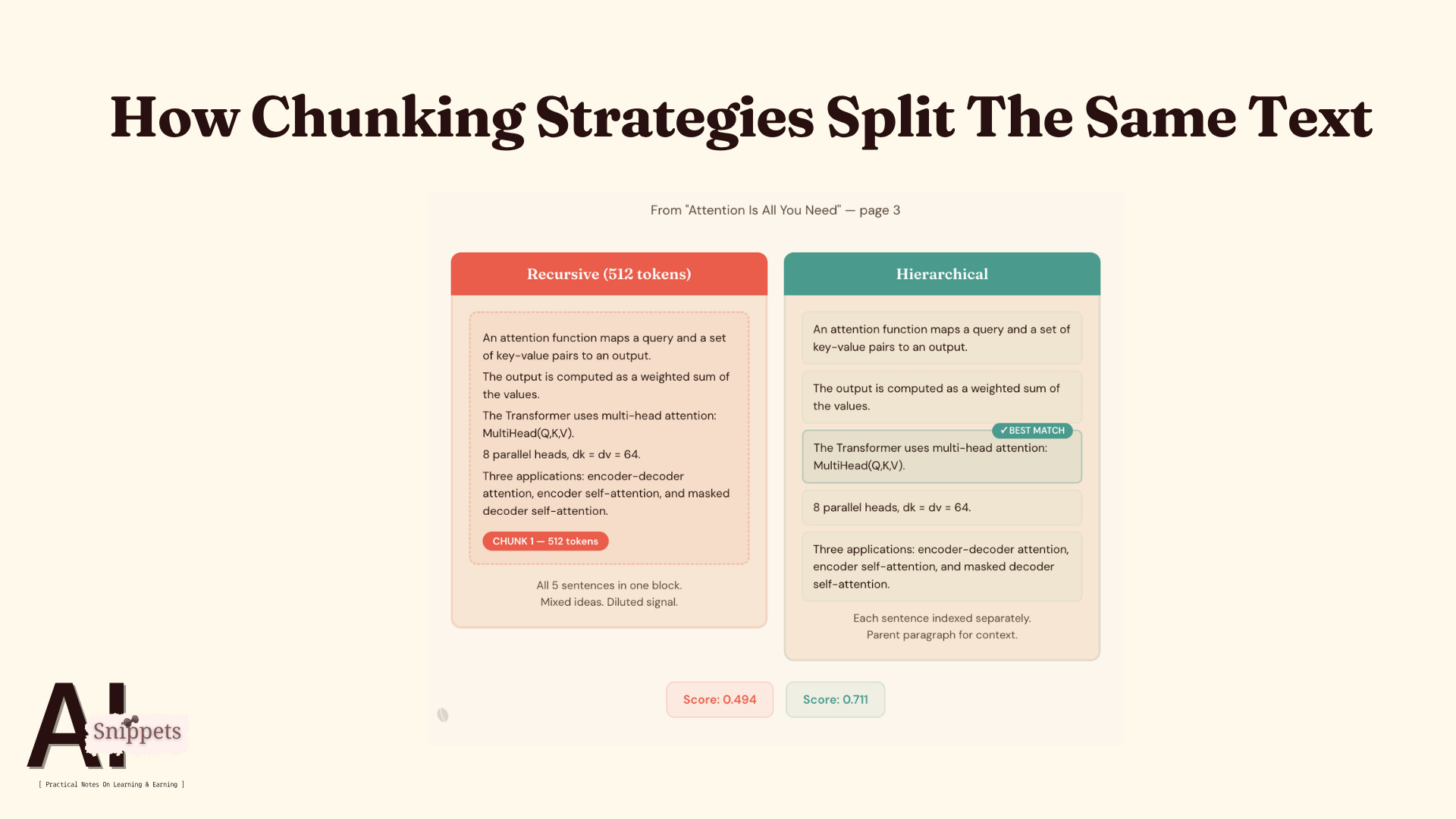
Retrieval scores jumped from 0.494 to 0.809.

The answer quality changed with it. One strategy surfaced the exact claim sentences from the papers. The other returned noise mixed with signal.

This issue is about that layer. The one between your model and your data. The one most builders skip. The one that determines whether your system is grounded or guessing.

In Issue 3, we said models are rarely the differentiator.

This is where the differentiator actually lives.

What The Retrieval Actually Is

Everyone talks about RAG.

Few talk about the system underneath it.

RAG is not a feature you add. It is a layer you design. And that layer has components most builders never think about independently.

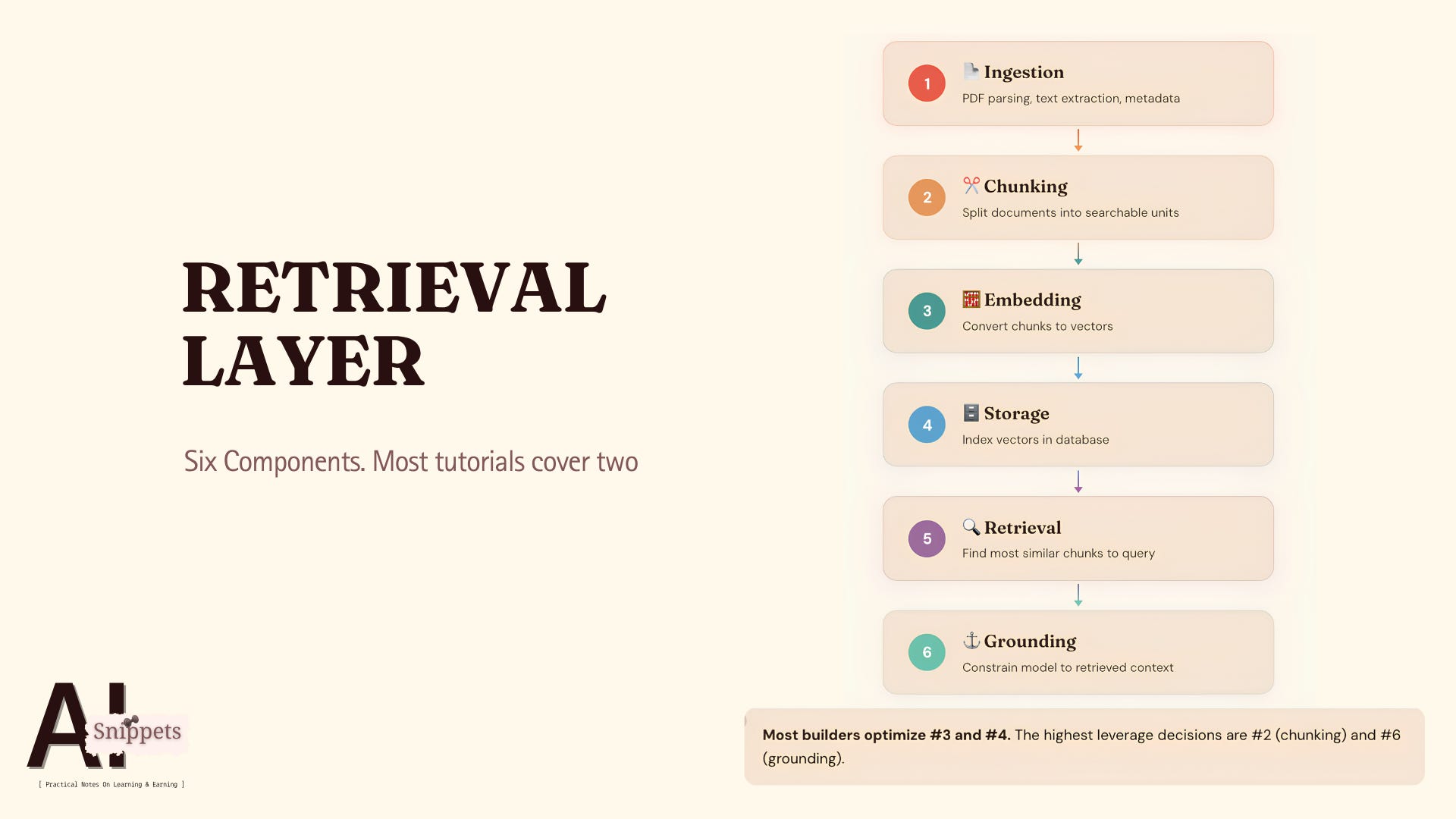
Here is what actually lives in the retrieval layer:

Ingestion. How documents enter your system. PDF parsing, text extraction, metadata tagging. Garbage in at this stage means garbage retrieved later. No model fixes bad ingestion.

Chunking. How documents get split into searchable units. This is the decision that determines retrieval quality more than any other. Most builders use the default. Most defaults are wrong for their data.

Embedding. How text chunks become vectors. The embedding model you choose shapes what “similarity” means in your system. A weak embedding model makes your vector database useless regardless of how much you paid for it.

Storage. Where vectors live and how they are indexed. ChromaDB for prototyping. pgvector when you already run PostgreSQL. Pinecone when you want managed infrastructure. The choice matters less than people think.

Retrieval logic. How your system decides what to surface. Top 5 by cosine similarity is the starting point. It is not the finish line. Reranking, filtering, hybrid search. This is where engineering shows.

Grounding. How retrieved context constrains the model’s output. Without grounding, your model generates fluently from nothing. With it, every claim traces back to a source.

Six components. Most tutorials cover two. Storage and a basic retrieval call.

The other four are where systems break.

And the one most builders get wrong first is chunking.

The Chunking Decision Nobody Talks About

Chunking is where most RAG pipelines silently fail.

Not loudly. Not with errors. The system runs fine. The retrieval returns results. The model generates an answer.

But the answer is shallow. Or slightly off. Or missing the one detail that mattered.

That is a chunking problem. Not a model problem.

Here is what chunking actually does. Your documents are too long to search as whole units. So you split them into smaller pieces. Each piece gets embedded as a vector. When a user asks a question, the system finds the pieces most similar to that question.

The question is: where do you split?

In 2026, the landscape has moved well beyond “pick a chunk size.” There are at least five serious approaches, each built for a different data problem.

Recursive splitting remains the production standard for roughly 80% of RAG applications. It tries to split at natural boundaries. Paragraphs first, then sentences, then words. You set a target size, usually 512 tokens with 10-20% overlap. It works. It is what most frameworks default to. It is what you are probably running right now.

Late Chunking processes the entire document through a long-context transformer before splitting. Every token’s embedding reflects the global context of the document. If a paper mentions “attention” on page one and refers to “the mechanism” on page eight, the embedding already encodes that relationship. Built for long, cross-referential documents like legal contracts and policy papers.

Adaptive Semantic Chunking (ASCM) uses dynamic programming to find mathematically optimal split points. It prevents breaking “protected entities” that must stay together. In oncology guidelines, it keeps a recommendation paired with its level of evidence. Built for structured medical, legal, and compliance documents.

W-RAC decouples extraction from planning at web scale. An LLM acts as a grouping planner using only structural metadata, not raw text. Built for organisations ingesting thousands of heterogeneous web pages. Solves a scale problem.

Hierarchical chunking (RAPTOR) creates layers of information. It indexes at the sentence level for precise matching, then retrieves the parent paragraph for context. It is the most widely adopted production retrieval pattern in 2025-2026 because it resolves the fundamental precision-context trade-off. Built for multi-hop reasoning where answers require connecting facts scattered across different sections or documents.

Five strategies. Each built for a specific data problem.

Choosing between them is not about picking the most advanced option. It is about matching the strategy to your data structure and query pattern.

For my test, the choice was specific.

Ten research papers. Cross-paper queries. Facts scattered across different documents. I needed to compare the production default against the strategy built for exactly this kind of multi-document retrieval.

Recursive vs hierarchical.

Not because the others are worse. Because these two are the comparison my data demanded.

The most cited chunking benchmark from early 2026 tested 7 strategies across 50 academic papers. Recursive scored 69% accuracy. Semantic chunking, the approach most tutorials position as “advanced,” scored 54%. Hierarchical was not included in that test.

That benchmark is useful as a starting point. It is not a substitute for testing on your own data.

In my pipeline, across 4 queries and 10 foundational AI papers, hierarchical won every time.

On a factual question about LoRA vs full fine-tuning, hierarchical scored 0.809. Recursive scored 0.559. Hierarchical latched onto the exact claim sentence: “LoRA performs on-par or better than fine-tuning in model quality.” Recursive returned a 512-token block where that sentence was buried among other content.

On a conceptual question about how AI agents use reasoning, the gap narrowed. Recursive scored 0.598. Hierarchical scored 0.673. The ReAct paper is dense with full conceptual paragraphs. When source content is already structured in paragraph-sized ideas, recursive does not lose as much signal.

And hierarchical had a weakness. It pulled in one off-topic chunk from the DeepSeek-R1 paper at 0.591. A sentence about “reasoning” in an unrelated context scored high enough to sneak in. Sentence-level precision can match too precisely on shared vocabulary.

One more thing worth noting. We used all-MiniLM-L6-v2 for embeddings in this test. It has a strict 256-token input limit. Our 512-token recursive chunks were silently truncated during vectorization. The second half of every recursive chunk was never embedded. The hierarchical strategy, which indexes at the sentence level, was largely unaffected by this limit because most sentences fall well under 256 tokens.

That asymmetry likely inflated the gap between the two strategies in our results. Upgrading to an embedding model with a longer context window would change the absolute scores. Whether it changes the relative ranking is an open question we will revisit in the next issue when we cover retrieval evaluation.

No strategy is universally best.

The right question is not “which chunking strategy should I use?”

It is “what does my data look like, what are my query patterns, and which strategy respects both?”

Most builders never ask that question. They use the framework default and move on. When retrieval underperforms, they blame the model.

The model was never the problem.

What The Scores Actually Mean

Most builders see a retrieval score and treat it like a grade.

0.8 is good. 0.4 is bad. Higher is better. Move on.

That intuition is wrong. And it leads to bad debugging decisions.

A retrieval score is a cosine similarity measurement. It tells you how close your query’s vector is to a chunk’s vector in embedding space. It ranges from 0 to 1. But the number alone means nothing without context.

Here is what I mean.

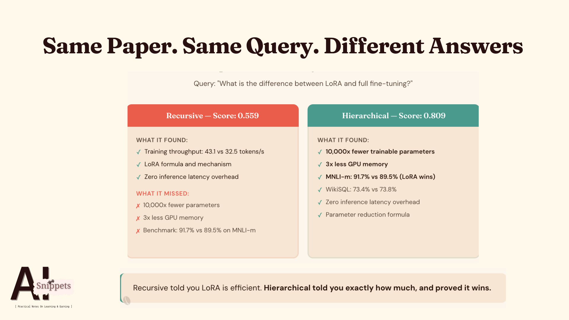
When I queried “What is the difference between LoRA and full fine-tuning?” the top hierarchical chunk scored 0.809. That is high because the query maps almost exactly to a sentence in the paper: “LoRA performs on-par or better than fine-tuning in model quality.”

The question and the answer use nearly the same words. The embedding vectors are close. The score reflects that.

When I queried “How does RAG reduce hallucinations compared to fine-tuning?” the top hierarchical chunk scored 0.509. The top recursive chunk scored 0.387.

Both scores are lower. Significantly lower. But the pipeline was not broken.

The papers do not frame “hallucinations vs fine-tuning” as a direct comparison. That framing exists in my question, not in the source text. The system had to find obliquely related content. It found it. The RAG paper’s discussion of factual accuracy on page 7. The LoRA paper’s performance comparisons.

Lower scores meant harder retrieval. Not failed retrieval.

The real signal was what happened next. Both answers correctly hedged. They acknowledged the context was indirect. They cited the specific pages they drew from. They did not fabricate a clean comparison that the source material never made.

That is the system prompt doing engineering work. “Answer only from the provided context. If the context does not contain the answer, say so.”

A weaker system prompt would have let the model fill in the gaps with training data. The answer would have sounded better. It would have been less trustworthy.

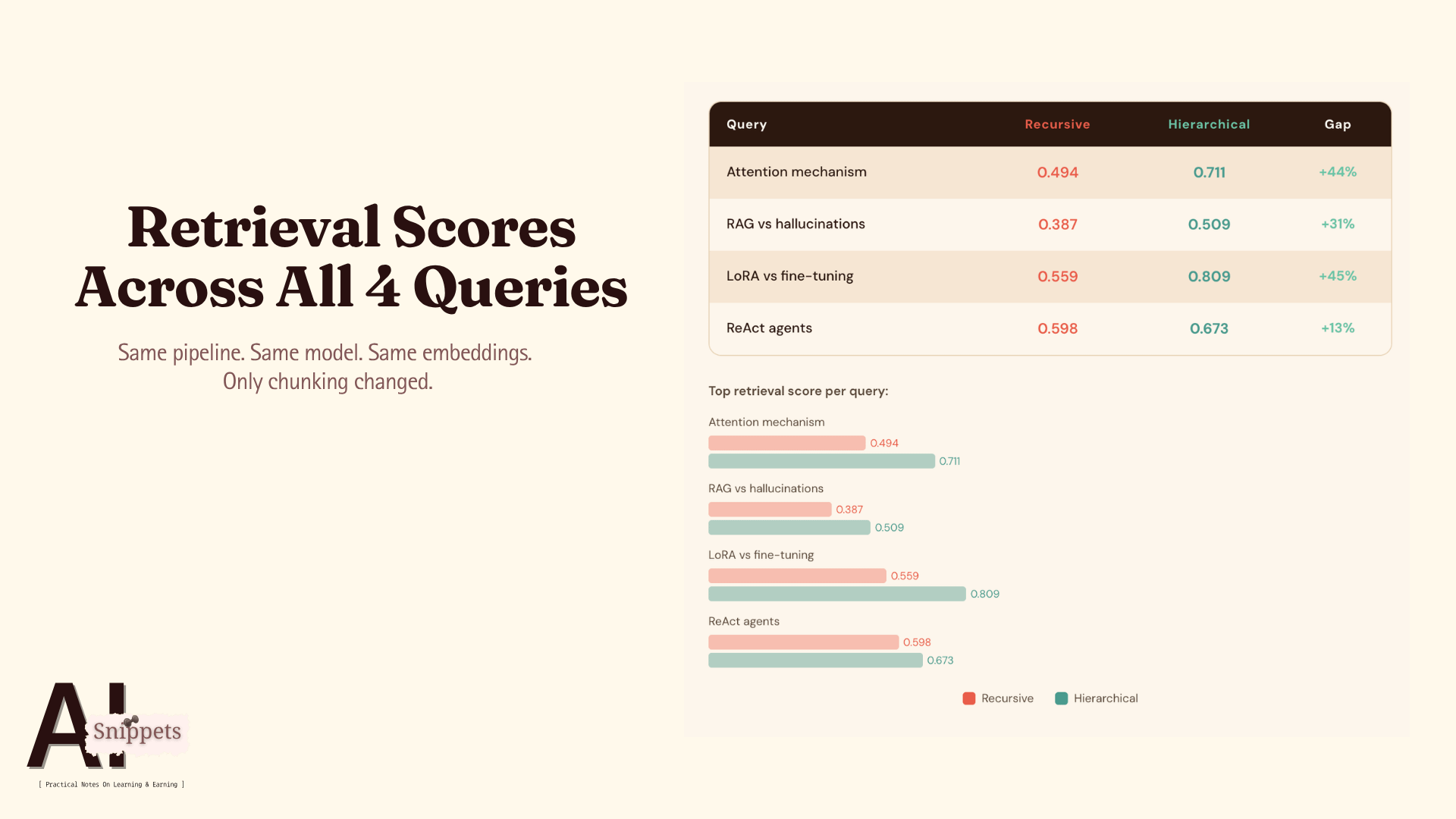
Here is the full picture across all four queries:

Query 1: Attention mechanism. Hierarchical 0.711. Recursive 0.494.

Query 2: RAG vs hallucinations. Hierarchical 0.509. Recursive 0.387.

Query 3: LoRA vs fine-tuning. Hierarchical 0.809. Recursive 0.559.

Query 4: ReAct agents. Hierarchical 0.673. Recursive 0.598.

Three patterns emerge from this data.

First, hierarchical consistently outscored recursive. The gap ranged from 13% to 45%. Sentence-level indexing finds better matches than block-level indexing. That held across every query type.

Second, the gap widened on factual questions and narrowed on conceptual ones. When the answer exists as a single clear statement in the paper, hierarchical finds it precisely. When the answer is distributed across a dense paragraph, recursive closes the gap because its larger chunks capture more surrounding context.

Third, absolute scores varied dramatically by query. 0.809 on LoRA. 0.387 on RAG vs hallucinations. Same pipeline. Same embedding model. Same vector database. The difference was how directly the question mapped to language in the corpus.

This is why a single retrieval threshold is dangerous. Teams set a cutoff. “Only return chunks above 0.5.” That works for queries that map cleanly to the source text. It silently drops valid results for queries that require indirect matching.

And thresholds are not portable. A cosine score of 0.5 on a 384-dimensional model like MiniLM means something entirely different on a 3072-dimensional model like text-embedding-3-large. The score distribution shifts with embedding architecture, dimensionality, and even the vocabulary distribution of your corpus. If you copied a threshold from a tutorial, it is almost certainly wrong for your pipeline. Evaluate per configuration.

The score is a signal. It is not a verdict.

If you are debugging retrieval quality, do not start by looking at the score. Start by looking at what was retrieved. Read the chunks. Check the citations. Ask whether the system found the right content, even if the score was low.

A 0.4 that retrieves the right paragraph is more valuable than a 0.8 that retrieves the wrong one.

Why Hierarchical Won (And Where It Didn’t)

The scores tell you which chunks were retrieved. They do not tell you what the model did with them.

Answer quality is where the chunking decision actually shows up. Two strategies can retrieve from the same paper, cite the same pages, and produce meaningfully different answers.

Here is where that happened.

On the LoRA query, both strategies pulled exclusively from the LoRA paper. Same source. Same pages. But the answers diverged.

Recursive surfaced training throughput numbers. 43.1 vs 32.5 tokens per second. It found the formula for how LoRA works. Technically correct. But it missed the headline.

Hierarchical found the two sentences that matter most. “10,000x fewer trainable parameters.” “3x less GPU memory.” Pulled directly from the abstract on page 1. It also surfaced the benchmark table showing LoRA beating full fine-tuning on MNLI-m: 91.7% vs 89.5%.

Recursive told you LoRA is efficient. Hierarchical told you exactly how much, and proved it wins.

The difference is mechanical. Recursive searches 512-token blocks. The abstract’s key claims share that block with methodology details, related work references, and formatting artifacts. The signal is there but diluted. The similarity score reflects the average relevance of the entire block, not the relevance of the best sentence inside it.

Hierarchical searches individual sentences. “LoRA reduces the number of trainable parameters by 10,000x” is a standalone unit of meaning. When that sentence matches a query about the difference between LoRA and full fine-tuning, the score is high because the match is direct. Then the system expands to the parent paragraph, giving the model enough context to generate a complete answer.

Small chunks for finding. Larger chunks for understanding. That is not a tagline. It is the mechanism.

On the attention mechanism query, the same pattern held. Both strategies found the right paper. But hierarchical surfaced the motivation behind multi-head attention: “with a single attention head, averaging inhibits this capability.” Recursive returned the architecture description without the reasoning behind it.

The model generated a technically correct answer from recursive chunks. It generated a more complete answer from hierarchical chunks. The difference was not intelligence. It was input quality.

On the RAG vs hallucinations query, hierarchical found the one concrete example in the entire corpus. When asked to “define middle ear,” BART produced a factually incorrect response. RAG models generated accurate anatomical descriptions. That example lives on page 7 of the RAG paper. Recursive never surfaced it. The 512-token block containing that example also contained surrounding discussion that diluted the match.

Hierarchical also found the human evaluation numbers. RAG was rated more factual 42.7% of the time vs BART’s 7.1%. Concrete evidence that recursive missed entirely.

But the ReAct query told a different story.

Hierarchical still won on score. 0.673 vs 0.598. But the gap was the smallest of any query. And hierarchical introduced noise that recursive avoided.

The ReAct paper is dense with conceptual paragraphs. Ideas are not expressed as single claim sentences. They are built across multiple sentences in tightly structured arguments. Recursive’s 512-token blocks captured these naturally. The larger window matched how the authors actually wrote.

Hierarchical still found the better answer. It surfaced the concrete Thought-Action-Observation loop, the pepper shaker example from the paper, and the hard benchmark numbers: 34% improvement on ALFWorld, 10% on WebShop.

One result worth noting. A sentence from the DeepSeek-R1 paper about "reasoning" in an unrelated context scored 0.591 and appeared at rank 5. It matched on vocabulary, not meaning. At rank 5 in a 10-paper corpus, this is noise, not failure. But in a larger corpus with hundreds of papers sharing similar terminology, this pattern could push relevant results out of the top-k window. Sentence-level matching is precise. That precision becomes a liability when your corpus has overlapping vocabulary across unrelated documents. Something to watch as the corpus scales.

Recursive had zero noise on this query. Every chunk came from the right paper.

Here is what this tells you.

Hierarchical is not universally better. It is consistently better for corpora where key insights exist as standalone statements. Research papers, documentation, technical specifications. Content where one sentence can carry a complete claim.

It is less dominant on dense, argument-driven text where meaning builds across paragraphs. Philosophy papers, legal arguments, narrative-heavy reports. Content where the unit of meaning is larger than a sentence.

And it introduces a specific risk: false matches on shared vocabulary across documents. If your corpus contains multiple papers that use similar terminology for different concepts, hierarchical will occasionally surface the wrong one.

The fix is not switching strategies. It is adding a reranking step. Retrieve with hierarchical precision, then rerank with a model that evaluates semantic relevance, not just vector similarity. That catches the vocabulary false matches without sacrificing the precision advantage.

But that is an optimization. Not a starting point.

The starting point is understanding what your data looks like and choosing the strategy that respects its structure.

The Decisions That Actually Matter

Most RAG conversations focus on vector databases.

Which one is fastest? Which one scales? Which one has the best pricing tier?

That conversation is backwards.

In my pipeline, I used ChromaDB. It runs locally. No account. No API key. No cost. It stores vectors in-process, so there is no network latency on queries.

For 10 papers and roughly 3,000 chunks, it is more than enough. For most prototypes and internal tools, it is more than enough.

The vector database was never a hard decision. Switching from ChromaDB to Pinecone or Weaviate would not have changed a single retrieval score in this test. Given the same vectors and the same query, every vector database returns the same nearest neighbours. The differences between them are operational: latency at scale, managed infrastructure, and metadata filtering. For retrieval quality, the vectors going in matter. The database storing them does not.

Here is what actually moved the needle, in order of impact:

Chunking strategy was the highest-leverage decision. Switching from recursive to hierarchical changed retrieval scores by 13-45% across every query. No other single change in the pipeline would have produced that difference. Not a better embedding model. Not a different vector database. Not a more expensive LLM.

The system prompt was the second-highest-leverage decision. “Answer only from the provided context. Cite which paper each claim comes from. If the context does not contain the answer, say so.” That constraint is what kept the model honest on the RAG vs hallucinations query. Without it, model would have generated a clean, fluent, wrong answer from training data.

Grounding is not a feature. It is a constraint you enforce.

Embedding model choice mattered less than expected, with a caveat. I used sentence-transformers (all-MiniLM-L6-v2). It runs locally. It is free. It is not the best embedding model available. Voyage AI’s voyage-3-large leads the 2026 benchmarks. OpenAI’s text-embedding-3-large is widely used in production.

For this corpus and these queries, a free local model was sufficient to demonstrate the chunking strategy difference. But there is a confounding variable. MiniLM has a 256-token input limit. Our recursive chunks were 512 tokens. That means half of every recursive chunk was silently truncated before it was ever embedded. This likely penalized recursive more than hierarchical, inflating the gap between the two strategies.

We will test this directly in the next issue by running the same pipeline with a longer-context embedding model and comparing results. Until then, the honest conclusion is: chunking strategy had a larger observable impact than embedding model choice in this test, but the two variables were not fully isolated.

Most builders optimize embeddings before they optimize chunking. That is still the wrong order. But both decisions compound, and testing them independently is part of the evaluation discipline we will cover next.

Model selection for generation was the lowest-leverage decision. I used Sonnet 4.6. Not Opus. For grounded generation from retrieved context, where the model’s job is to synthesize provided chunks and cite sources, Sonnet performs within 1-2% of Opus at 40% lower cost.

Opus earns its price on tasks that require deep reasoning without provided context. RAG generation is not that task. The context is provided. The model synthesizes. Sonnet does this well.

If your pipeline retrieves the right chunks, almost any capable model generates a good answer. If your pipeline retrieves the wrong chunks, no model saves you.

Retrieval quality is upstream of everything.

Here is the order most builders follow:

1. Pick the best model

2. Pick a vector database

3. Add RAG

4. Wonder why it hallucinates

Here is the order that works:

1. Design your chunking strategy for your data

2. Enforce grounding through system prompt constraints

3. Choose an embedding model appropriate to your scale

4. Pick a generation model appropriate to the task complexity

5. Choose a vector database appropriate to your infrastructure

The sequence matters. Each decision constrains the ones after it. Most builders start at the bottom of the stack and work up. Engineers start at the top.

That is the retrieval layer. Not a database choice. A system design.

What’s Next?

The retrieval layer answers one question: what does the system know?

Not what the model was trained on. What your system can access, retrieve, and ground its responses in. That is the difference between fluency and reliability. Between a demo and a product.

When this layer works, every layer above it gets stronger. Orchestration becomes predictable because the data feeding each step is trustworthy. Deployment becomes stable because outputs are grounded, not generated from nothing. Evaluation becomes possible because every claim traces back to a source.

When this layer is weak, every layer above it compensates. The model guesses. The orchestrator retries. The user loses trust. And the team blames the LLM.

Most RAG failures are retrieval failures. Not model failures.

That is the core lesson from this build. Same model. Same vector database. Same queries. One change in the chunking strategy shifted what the system surfaced. Recursive returned relevant chunks with the evidence diluted inside them. Hierarchical surfaced the specific claims directly.

The exact size of that gap has a caveat. Our embedding model truncated the longer recursive chunks, likely inflating the difference. We will isolate that variable in Issue 4b.

But the direction is clear. The model never changed. The system around it did. And retrieval was the layer that made the difference.

If you are building RAG right now and the outputs feel unreliable, do not start by switching models. Start by reading the chunks your retriever is actually returning. Check whether the right content is reaching the model before you blame the model for the wrong answer.

The retrieval layer is not glamorous. It does not make headlines. Nobody posts about their chunking strategy on social media.

But it is where grounding lives. And grounding is what separates systems that work from systems that perform.

But this issue left one question open.

We flagged a confounding variable. Our embedding model silently truncated half of every recursive chunk. The gap between strategies may be real, inflated, or somewhere in between. We do not know yet because we have not isolated the variables.

That is an evaluation problem. And most builders never run the test.

Next issue, we stay in the retrieval layer.

Issue 4b is about retrieval evaluation. How to measure whether your pipeline is actually working. How to isolate chunking from embedding from retrieval logic. How to know whether a score means something or nothing.

We will re-run this exact pipeline with a longer-context embedding model and compare results. Same papers. Same queries. Different embeddings. The test we owe ourselves before making any confident claims.

Retrieval without evaluation is guessing with extra steps.

Issue 4b removes the guessing.

This issue is part of our on-going series. Here's the full series.

Series Navigation

• Issue 1: The Difference Between AI Learners and AI Engineers

• Issue 2: The First Skill AI Engineers Build

• Issue 3: The Model Layer: Why Intelligence Is Rarely the Differentiator

• Issue 4a: The Retrieval Layer — Chunking ← you are here

• Issue 4b: The Retrieval Layer — Evaluation (coming next)

• Issue 5: The Orchestration Layer

• Issue 6: The Deployment Layer

• Issue 7: The Observability Layer

• Issue 8: The Full Stack: Putting It All Together

If you are building RAG systems and unsure whether your retrieval layer is the bottleneck, reply to this email with what you are building. I read every response.